Month: June 2024

Apple Intelligence in Europe doesn’t (yet) make sense

Apple’s decision not to introduce Apple intelligence, iPhone Mirroring, or SharePlay Screen Sharing in the European Union this year isn’t surprising, and reflects concerns around privacy far more than being a response to Europe’s decision to act against Apple’s App Store compliance.

The news basically is that Apple has confirmed it will not introduce the Apple Intelligence features it announced at WWDC in EU nations because it has concerns around the application of the Digital Markets Act (DMA). 

Apple Intelligence delayed, App Store gets a DMA slap

“Due to the regulatory uncertainties brought about by the Digital Markets Act, we do not believe that we will be able to roll out three of these [new] features — iPhone Mirroring, SharePlay Screen Sharing enhancements, and Apple Intelligence — to our EU users this year,” Apple told the Financial Times.

At the same time Apple made its announcement, the EU itself announced it will begin to take enforcement action against the company for breach of the DMA. Europe is concerned about elements of Apple’s offer to developers and the fees it charges the small number of developers who are the most successful on the store, arguing this stifles competition. Apple says it has made changes and is “confident” its plans align with that law.

It’s worth noting that the EU recently proposed an incredibly intrusive surveillance law that would break end-to-end encryption. While it looks like those proposals may have been shelved, Apple might have decided to stall while it waits to see what kind of shabby surveillance laws do get passed. 

Privacy or convenience? It’s up to EU

If you think about it, the beauty of Apple Intelligence is that it uses information your device has collected about you in order to function. But the risk of that information existing — even on your device — is that under the DMA, it’s not certain the EU won’t insist on that data, your data, being opened up to competitors. 

That’s a lot of information.

Apple is committed to keeping that information private and secure, but once it exists and is on the device in some form, I expect the company is concerned the DMA could force it to open up the information to third parties who want to compete with their own AI. As we’ve seen since the invention of the Internet, not every company is legitimate, ethical, or trustworthy, and even those that are might not have enough clout to invest in the world’s best security teams to maintain safety on their platforms.

A Pandora’s box chock-full of trouble

I get the sense that Apple’s decision to hold back on Apple Intelligence in the EU reflects the ongoing battle between the two entities as Europe forces Apple to open up a little. Given the source of this speculation, that might be correct, but the analysis misses what’s really at stake: once you have all your personal information turned into usable data on your device, every spook, hacker, fraudster, blackmailer, censor, despot, cop, or secret service operative is going to want to take a look.

That means any weakness in protecting that information opens a Pandora’s box of misanthropy — affecting consumers, corroding trust, and enabling surveillance at a scale no one has seen ever before on our sadly ailing planet. 

Could the EU end up without Apple Intelligence? 

It feels possible EU might never get Apple Intelligence.

Apple says: “We are committed to collaborating with the European Commission (EC) in an attempt to find a solution that would enable us to deliver these features to our EU customers without compromising their safety.”

According to the Financial Times, Apple seeks “clarity” from the European Commission regarding the level of access it would need to grant to third parties over Apple Intelligence features in order to be DMA-compliant.

However, rather than providing any insight into requirements, an EU rep said companies like Apple are, “Welcome to offer their services in Europe, provided that they comply with our rules aimed at ensuring fair competition.” Which is, of course, what Apple is asking for, it just wants to know how those rules will be applied to its service before launch, rather than working with decisions made after the event.

What isn’t yet clear is the extent to which other AI providers might be affected. Is it possible the European Commission might have just created an obstacle to AI deployment?

Who has the energy for this?

And, of course, the big conversation everyone should be having concerning artificial intelligence is one Europe’s regulators don’t appear to be addressing at all — the energy consumption of AI servers. Combined, the world’s data centers now consume more power in a year than the entire Italian nation, and this is set to increase exponentially. Perhaps waiting until privacy, security, and energy challenges are solved makes sense after all?

One more thing is also certain: That with the removal of these three features the temptation to upgrade to iOS 18 among European users will be lower than ever before, given they comprise the majority of improvements to the OS.

Please follow me on Mastodon, or join me in the AppleHolic’s bar & grill and Apple Discussions groups on MeWe.

AI is starving for more power. Can quantum computing help?

Data centers are draining more electricity from global power grids than ever before because of generative artificial intelligence (genAI) and general AI processing needs. 

The compute capacity to train large language models, the platforms on which generative AI (gen) and AI run, is now roughly doubling every nine months, according to Epoch AI, an AI research institute. The International Energy Agency forecast that global data center electricity demand will more than double from 2022 to 2026, in large part because of AI and cryptocurrency.

That insatiable demand for energy has tech companies scrambling for alternative sources of energy as well as ways to reduce the energy needs of AI technologies.

One potential emerging solution to the AI-compute dilemma is quantum computing, which vastly surpasses today’s binary computing systems in processing capabilities and energy consumption. Studies have shown quantum computing can increase the performance of AI neural networks for tasks such as natural language processing and image analysis.

“Quantum computing definitely augments the power of AI. For example, AI and quantum computing used together can accelerate drug discovery and personalized pharmaceuticals by years. Quantum computing supports AI-based simulation of clinical drug trials so that the trials take one hour instead of ten years,” said Avivah Litan, a vice president analyst at Gartner.

For example, in February, Insilico Medicine and the University of Toronto announced they’d demonstrated the first instance of a generative model running on quantum hardware outperforming state-of-the-art classical models in generating viable cancer drug candidates.

What is quantum computing?

In classical computers, bits programmed as units of data have a possible value of one or zero — hence the term binary code. In quantum computers, data units are programmed with quantum bits, known as qubits, which can represent a one, a zero, or a combination of both zero and one at the same time. At a high level, that trait enables quantum computers to be faster and better at fundamental processing tasks than data processing on classical computing systems that use GPUs or CPUs.

For example, Google’s Quantum AI division built a supercomputer based on its Sycamore quantum processor. Each chip currently holds 70 qubits and can reportedly complete in seconds what would take a CPU- or GPU-based supercomputer of similar size decades to process.

Google Sycamore processor

From left to right, Google’s rendition of its Quantum computing platform and its Sycamore quantum processor.

Google

“Quantum artificial intelligence with better algorithms… are faster and more accurate,” CompTIA, a global, nonprofit IT association, stated in a blog.

Commercial quantum platforms, such as Microsoft Azure Quantum, AWS Braket, Google Cirq, and others, allow cloud providers to use quantum comuting as compute service offerings.

“Think of these platforms as quantum computing marketplaces whereby the cloud service providers have partnered with multiple quantum computing vendors to provide access to their hardware, software, QSDKs [Quantum software development kits], etc.,” said Heather West, a research manager with IDC.

“Most of these cloud service providers have not, and thus do not, provide access to their own quantum systems, the exception being Google. AI is not a part or related to these offerings,” she added.

As with any technology, along with the positives there are negatives associated with quantum computing. For example, quantum computing poses a serious threat to the cybersecurity systems relied on by virtually every company, according to CompTIA. The current standard for encryption algorithms, such as RSA or SSL/TLS, relies on the complexity in factoring large numbers into primes, and that’s the type of problem quantum computers are great at solving, CompTIA said.

Startups and established companies continue to accelerate their advances in the quantum computing space. Big tech companies such as Alibaba, Amazon, IBM, Google, and Microsoft have already launched commercial quantum-computing cloud services. Two years ago, Goldman Sachs said it planned to introduce quantum algorithms to price financial instruments as soon as 2026. Honeywell anticipates that quantum will form a $1 trillion industry in the decades ahead.

Quantum computing, meet genAI

Some say quantum computing is a natural partner for genAI and can reduce its energy demands.

For example, Sumitomo Mitsui Trust Bank in Japan is using quantum computing to run genAI-powered programs for financial simulation models of future market movements. The bank partnered with Zapata AI, a genAI company that was spun out of Harvard University’s quantum computing lab in 2017.

Christopher Savoie, Zapata AI’s CEO, sees linear algebra (quantum math) as the solution to perform all kinds of AI tasks, including chatbots such as ChatGPT.

“We’re throwing an obscene the amount of GPU energy at chatbots right now. Are we getting that much business value right now from it? We’re hitting a wall: when are we going to make money with that?” said Savoie, who is a molecular biophysicist.

Savoie pointed to the study done by Insilico Medicine and the University of Toronto, which Zapata participated in.

“When we used this quantum-based model… we were able to develop cancer drugs the other models didn’t,” Savoie said. “We used quantum models to determine what drugs would block this cancer protein and then non-quantum models. The quantum models found two capable drugs that we synthesized and showed they blocked the cancer protein.

“So, it’s qualitatively better,” he continued. “It’s cheaper, faster, and better — better in that we get faster answers. That’s important in drug discovery. You’re saving a lot of money for pharmaceutial companies if you get your answer the first run around. Or you have a more accurate modeling of trading behavior for a bank.”

Zapata AI’s Orquestra platform was specifically designed to run any AI or machine learning model, including more traditional neural networks as well as the company’s proprietary tensor networks.

Tensor networks can be used to model any quantum circuit and run it on today’s classical computers, giving users an on ramp to the potential benefits of future quantum computers, according to Zapata AI. Tensor networks also come with their own advantages for AI today, including more accurate, efficient, and expressive AI models.

“Every quantum circuit can be written as a tensor product, which means we can do things on GPUs that quantum computers will eventually be faster at doing. Zapata and others have shown that quantum math is better at getting better answers in the context of generative AI,” Savoie.

Specifically, Savoie said, quantum statistics can enhance genAI models’ ability to extrapolate missing information and generate new, high-quality information from big data. Generating genuinely new and high-quality data is very important for industrial use cases, he said. 

Early days yet

IDC’s West said quantum computing fits with complex problem solving, but it’s “not a big data solution.” Quantum computing will be useful for solving specific types of problems, she said.

In quantum computing, a qubit begins in a binary state of 0 or 1, but through a process known as annealing, the qubits become entangled, allowing them to represent many possible answers, always with minimum energy. The process occurs in microseconds.

“Quantum annealers are best suited for optimization problems,” West said. “The complex algebraic/factorization problems include some QML [quantum machine learning] problems, but not all AI problems will be suitable for quantum. Research is being conducted to determine how to integrate AI into [quantum computing] and [quantum] into AI to optimize the compute resources needed to solve some of these problems.”

In large part, quantum computing is in very early stages of development, West noted. That’s because the hardware still needs considerable improvements for gate-based models that allow for the​ execution of quantum‌ algorithms. By applying various gates ​sequentially, complex computations can be carried out.

“There are not any real-world applications for this type of system,” West said. “These systems are only useful for small-scale experimentation and debugging. Quantum [computing is] currently being used for solve some scientific and business optimization problems. It is still too early for the integration of AI. Right now, it is only a hypothetical and experimental.”

SoundHound AI buys online food ordering platform Allset

SoundHound AI has enhanced its AI-based food ordering capabilities with the acquisition of Allset, an online ordering platform that connects restaurants and local customers.

Financial terms of the deal, announced Thursday, were undisclosed.

Allset is a food ordering platform designed for local pick-up, working with nearly 7,000 restaurant partners nationwide, including Joe & The Juice and Charleys Cheesesteaks.

Speech-to-meaning

SoundHound, a voice AI and speech recognition company, which was founded in 2005 went public in 2022. The company develops speech recognition, natural language understanding, music recognition, and search technologies.

In 2023, SoundHound generated $45.9 million in revenue, a 47% year-on-year increase. The vendor is growing but not yet profitable.

As part of Nvidia’s broader strategy of investing in AI-related tech companies the chip maker has invested $3.7 million into SoundHound, in return for a 0.6% stake.

SoundHound’s Vehicle Intelligence product, powered by Nvidia Drive, allows drivers to ask questions related to maintenance, safety and other vehicle-specific information using natural speech.

SoundHound markets itself as an independent voice AI platform, offering customers the ability to create their own branded voice experiences rather than relying on voice assistants from bigger vendors.

Allset

SoundHound said the deal to buy Allset will advance its plans to enable voice-enabled food and drink ordering across millions of cars, TVs, and smart devices. Its voice ordering technology works across multiple channels, including via phone, drive-thru, kiosk, and mobile app.

More than 10,000 restaurant locations use SoundHound’s platform to understand speech in a range of major languages, learn any restaurant’s menu, process orders directly to the point of sale (POS), and answer customer FAQs.

“Allset will help SoundHound bring voice AI solutions to even more restaurants looking to improve operational efficiency,” Keyvan Mohajer, CEO and co-founder of SoundHound AI, said in a statement on the deal.

For example, SoundHound has been working with White Castle, the US-based fast-food hamburger joint, to offer voice AI ordering technology at select White Castle drive-thrus for a year, with plans to roll out the technology to 100 locations by the end of 2024.

Many in the fast-food industry and looking to use AI technology to increase efficiency and reduce costs.

Using an AI system that provides a consistent, interactive ordering experience is a big ask.

Super size snags at McD’s

McDonald’s recently ended its trial of AI-powered drive-thru technology developed in partnership with IBM. McDonald’s had been testing IBM’s AI-powered voice recognition technology at around 100 US drive-thru locations for around two years.

The technology has numerous glitches, chiefly around the misinterpretation of customers’ orders to sometimes comical effect.

Hard to swallow mistakes including adding bacon to ice cream and putting excessive quantities of items on orders (e.g. hundreds of chicken nuggets on a single order). People took to social media with tales of “fighting the McDonald’s robot” and similar.

The automated order taking system — which evidently had problems picking up on accents and dialects, noise and cross-talk from neighbouring drive-thru stations – will be dropped from the end of July, Restaurant Business reported.

IBM is yet to respond to a request for comment from Computerworld but reportedly said it looks forward to working with the fast food restaurant chain on a variety of project in the future.

Bill Conner, CEO of mobile technology developer Jitterbug, told Computerworld that teething problems with new technologies are to be expected. Waiting for technologies to mature is unwise since slow adoption of AI technology is likely to leave businesses at a competitive disadvantage, Conner argued.

“The future of application development, orchestration and automation is based on an AI evolution, not a revolution,” Conner said. “Even the most agile organizations need a smart, measured approach to infusing AI capabilities into their business and infrastructure.”

In today’s enterprise, Apple hits the DEX

As employee experiences become increasingly digitized, the digital employee experience (DEX) is becoming the primary interaction you and your workers have, whether in person, remote, or hybrid. That’s why the technologies that enable whatever mission you happen to be on have become so important, as the tech is by definition an essential component in any digital employee experience.

We know because they told us

We already know this because big enterprises like SAPSalesforceCiscoIBM, and many others have told us that when given the choice, employees will choose an Apple product as their primary workplace device. We also know that, for example, sales of portable Macs absolutely boomed during the pandemic, when every office-based worker transitioned to become a home-based employee in a matter of weeks. 

Once the pandemic seemingly ended, those home-based workers became mobile employees, and later — sometimes reluctantly — turned into hybrid workers. 

In that sense, the importance of Apple’s products has already been proven. These devices, whether Mac, iPhone, or iPad, have already been used on a global scale to maintain businesses remotely in real time — as will visionOS devices in their time. 

That success continues to translate into increasingly large deployments across industries you might not have considered to be natural Apple users before, from retail to engineering and beyond. 

Empowering good business with DEX

Of course, business leaders recognize the changing workplace, with 24% of leaders already seeking to unlock improved DEX and productivity. The analysts at Gartner say digital workers who are happy with the tools and applications provided for work are 1.6 times more likely to stay.

While not everyone is an Apple user, sundry TCO studies suggest that businesses that do adopt those products realize significant benefits in terms of support costs, device longevity, employee retention, and productivity.

But at its core, Apple’s key offer to business is the same one it offers to consumer users: a user interface that, for the most part, gets out of the way to enable the user to get what they want to get done as effectively as they can.

That’s the whole point of smart DEX strategy — to equip and empower employees so they can stay focused on their task and not get bogged down by tech.

This secret sauce is compelling to any busy person, and the savor gains gusto on strength of Apple’s full platform — by which I mean that on mobile, tablet, or computer you get a similar DEX.

This familiarity is critical, as it makes it easier to complete tasks on whatever device makes the most contextual sense for a person at any point in time. In essence, the provision of consumer-simple technologies capable of delivering enterprise-class results to employees who can work from anywhere empowers immense business flexibility. 

Infrastructural change

The other post-pandemic benefit supporting the trend comes through the rapid evolution of device management of Apple devices since the pandemic first hit.

Sure, there was already a healthy industry of device management vendors (including Apple itself), but the company took note of enterprise pain points and introduced tools to address them. Think zero touch, declarative device management, improvements to activation lock, and even the recent introduction of a dedicated (and provisionable) password app based on the company’s existing iCloud Keychain. 

The result? 

At the front end of business, DEX improves through employee-driven adoption of Apple’s products.

But the company has also been speaking with both Windows- and Apple-familiar IT admins to figure out how to enable good experiences for them. It’s now truly possible to ship hardware to new hires, who can safely and effectively start their managed employee experience with a single login to their new device — and for IT to manage the entire transition through a single pane of glass.

Please follow me on Mastodon, or join me in the AppleHolic’s bar & grill and Apple Discussions groups on MeWe.

Anthropic Claude 3.5 Sonnet is here, and it’s free

Anthropic, the AI startup that claims to differentiate itself from its peers as a responsible AI firm, launched a new AI model — Claude 3.5 Sonnet. This is the first model in its anticipated Claude 3.5 series and the company claims it surpasses current industry standards in AI intelligence.

Anthropic is offering Claude 3.5 Sonnet for free on Claude.ai and the Claude iOS app, while it would allow Claude Pro and Team plan subscribers to access it with significantly higher rate limits. Claude 3.5 Sonnet is also available via the Anthropic API, Amazon Bedrock, and Google Cloud’s Vertex AI.

This announcement builds upon Anthropic’s previous releases — Claude 3 Haiku and Claude 3 Opus.

“Claude 3.5 Sonnet is now available for free on Claude.ai and the Claude iOS app, while Claude Pro and Team plan subscribers can access it with significantly higher rate limits,” an Anthropic announcement noted.  “It is also available via the Anthropic API, Amazon Bedrock, and Google Cloud’s Vertex AI.”

More power, less cost

Anthropic claimed that Claude 3.5 Sonnet surpasses competitor models like GPT4.o and Gemini 1.5 Pro, Meta’s Llama 3 400B, and even its predecessor, Claude 3 Opus, on a wide range of evaluations. Notably, the Claude 3.5 Sonnet achieves this leap in performance while maintaining the speed and cost-effectiveness of their mid-tier model, the Claude 3 Sonnet.

“The Claude 3.5 Sonnet represents a significant advancement in large language models, featuring notable improvements across key metrics,” said Prabhu Ram, head of the Industry Intelligence Group at CyberMedia Research. “It boasts double the processing speed of its predecessor, Claude Opus, at a fraction of the cost.”

Claude 3.5 Sonnet sets new industry benchmarks for graduate-level reasoning (GPQA), undergraduate-level knowledge (MMLU), and coding proficiency (HumanEval), Anthropic said. “It shows marked improvement in grasping nuance, humor, and complex instructions, and is exceptional at writing high-quality content with a natural, relatable tone.”

The company claimed that Claude 3.5 Sonnet operates at twice the speed of Claude 3 Opus. This performance boost, combined with cost-effective pricing, “makes Claude 3.5 Sonnet ideal for complex tasks such as context-sensitive customer support and orchestrating multi-step workflows.”

As per the announcement, the new model costs $3 per million input tokens and $15 per million output tokens, with a 200K token context window.

In April the company launched Claude 3 Haiku as the most cost-effective AI solution with a fee of $0.25 per million token for input and $1.25 for output.

In terms of power and efficiency, Anthropic offers three versions of its Claude AI model — Haiku is the lightweight version while Sonnet and Opus are the middle and high-end models respectively.

Claude 3.5 Haiku and Claude 3.5 Opus are slated for release later this year, the announcement said.

Coding and vision capabilities get a boost

The announcement highlights Claude 3.5 Sonnet’s prowess in code manipulation and understanding. In an internal evaluation, the model solved 64% of problems related to bug fixing and functionality additions with open source codebases, a significant improvement over Claude 3 Opus’ 38% success rate.

“Our evaluation tests the model’s ability to fix a bug or add functionality to an open source codebase, given a natural language description of the desired improvement,” the announcement read. “When instructed and provided with the relevant tools, Claude 3.5 Sonnet can independently write, edit, and execute code with sophisticated reasoning and troubleshooting capabilities. It handles code translations with ease, making it particularly effective for updating legacy applications and migrating codebases.”

Claude 3.5 Sonnet also sets new standards for visual reasoning tasks, surpassing Claude 3 Opus in interpreting charts and graphs and accurately transcribing texts from imperfect images.

“Claude 3.5 Sonnet is our strongest vision model yet, surpassing Claude 3 Opus on standard vision benchmarks,” Anthropic claimed. This capability is particularly crucial for industries such as retail, logistics, and financial services, where visual data holds more insights than text.

Collaborative work environment gets a new name: Artefacts

Alongside Claude 3.5 Sonnet, Anthropic has launched a new feature called Artefacts on Claude.ai. This feature allows users to generate content such as code snippets, website designs, text documents, which appear in a dedicated window alongside their conversation. This creates a dynamic workspace where users can see, edit and build upon Claude’s creations in real-time, marking a significant evolution from conversational AI to a collaborative environment.

“This preview feature marks Claude’s evolution from a conversational AI to a collaborative work environment,” Anthropic stated in the announcement. “It’s just the beginning of a broader vision for Claude.ai, which will soon expand to support team collaboration.”

Soon, teams — and eventually entire organizations — will be able to securely centralize their knowledge, documents, and ongoing work in one shared space, with “Claude serving as an on-demand teammate.”

This feature marks a shift in Claude’s role, evolving from a conversational AI to a collaborative work environment.

The company is also developing new modalities and features to support more business use cases, including integrations with enterprise applications and personalized features like Memory which will enable Claude to “remember a user’s preferences and interaction history,” the announcement said.

Excel basics: Get started with tables

Tables are one of the fundamental tools in Excel. Putting your data in a table makes it visually appealing and much easier to read.

Tables also make it easier to work with your data, offering built-in sorting and filtering tools as well as easy-to-use calculation features to help you get useful insights from your data. In fact, some advanced Excel features, such as its new genAI-powered data analysis, require you to put your data in table format first.

In this story, we’ll get you up and running with tables in Excel, from creating and formatting them to performing calculations on their data. Below is the sample data we will be using, if you’d like to copy and paste it into a blank Excel worksheet and follow along with the tutorial:

ItemJanFebMarch
Lemons$300$220$240
Bananas$190$190$170
Apples$220$170$120
Pears$170$200$190

We’ll demonstrate in Excel for Windows with a Microsoft 365 subscription. If you use a different version of Excel, most steps will work similarly, but you may not have all the features shown here.

How to make and format a table in Excel

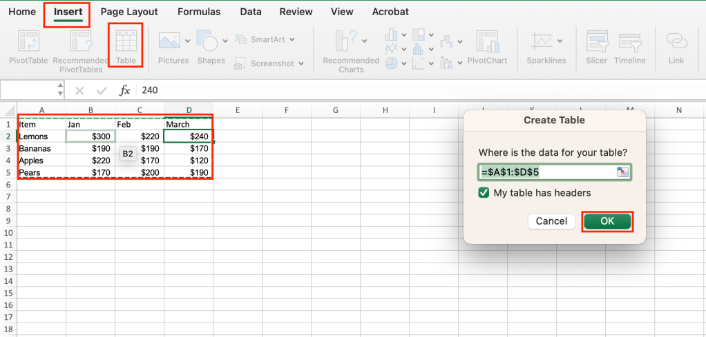
To create a table in Excel, go to the Insert tab on Excel’s Ribbon toolbar and select Table. The Create Table pane will pop up asking you to select the data you want to include in the table. Highlight the data you want in the table. If your data includes column headers (as our example does), click the My table has headers checkbox, and then select OK.

creating a table in excel

Creating a table in Excel.

Shimon Brathwaite / IDG

Alternatively, you can start by selecting the data you want to include in the table and then selecting Insert > Table. The Create Table pane will pop up with the data range prepopulated.

After you click OK, the table will appear in place of the plain data you selected. By default, the table will typically be formatted with a dark blue header and alternating light blue and white rows, but you can choose between several different colors and designs. To do so, click on the table you created, select the Table tab in the Ribbon, and scroll through the table design options at upper right. Click on any design, and your table’s formatting will instantly change to match. For this demonstration, we’ll select the yellow coloring.

formatting a table in excel

Choose a table design from the gallery on the Table tab.

Shimon Brathwaite / IDG

And that’s it. It took all of 20 seconds to create and format a table in Excel.

How to use a Total row for quick calculations

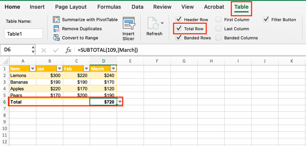
Next, you’ll add calculations to your table. This lets you summarize information easily for viewing. To do so, click on your table, navigate to the Table tab in the Ribbon, and check the Total Row option. A row marked “Total” appears at the bottom of the table. By default it shows the sum of the numbers in the final column of your table.

total row at the bottom of a table

Adding a Total row to the bottom of the table.

Shimon Brathwaite / IDG

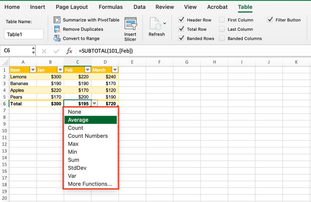
What if you want to show totals for the other columns in the table — or show something other than sums in the final row? Based on the name, it would seem that you can only use the Total row for totals, but that is not true. If you click in any cell in the final row, a downward pointing triangle icon appears next to it. Click the triangle and a dropdown appears. You can calculate many different values, such as average, minimum, maximum, standard deviation, and more, and you can calculate each column.

total row dropdown options

The Total row can perform many different types of calculations.

Shimon Brathwaite / IDG

If you choose to show calculations for multiple columns in a table, you’ll want to use the same calculation for each one so they’re consistent across the Total row. You’ll also want to label the row appropriately. If you’re showing averages in the Total row, for instance, change “Total” to “Average” in the first cell.

How to sort and filter data in an Excel table

In addition to making calculations, tables allow you to easily filter or sort data so that it can be presented in the way that you like.

Sorting

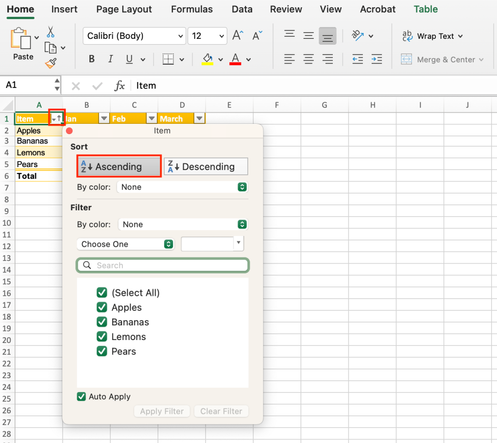
To sort items by ascending or descending order, simply click the downward triangle next to any column header and select Ascending or Descending on the pane that appears. If you’ve chosen a column with text, the rows will be arranged from A to Z or from Z to A. If you sort on a column with numbers, they’ll be arranged from lowest to highest or from highest to lowest.

sorting in ascending order

Sorting column A in ascending order.

Shimon Brathwaite / IDG

Sorting on a column brings the whole row along. In our sample data, for instance, sorting on column A in ascending order moves Apples to the top row — and the Jan, Feb, and March sales figures for Apples also move to the top row. This keeps all the relevant data together.

Filtering

You can also filter out some items completely to limit what is shown. This doesn’t delete any of the table data; it simply hides it so you can zero in on a subset of your data.

To do so, click the button next to the column header and then find the list of items in the column near the bottom of the pane that appears. Uncheck items until only the desired ones are left (in our case, Apples and Bananas).

srcset="https://b2b-contenthub.com/wp-content/uploads/2024/06/excel-tables-06-filter-by-name.png?quality=50&strip=all 1362w, https://b2b-contenthub.com/wp-content/uploads/2024/06/excel-tables-06-filter-by-name.png?resize=300%2C292&quality=50&strip=all 300w, https://b2b-contenthub.com/wp-content/uploads/2024/06/excel-tables-06-filter-by-name.png?resize=768%2C747&quality=50&strip=all 768w, https://b2b-contenthub.com/wp-content/uploads/2024/06/excel-tables-06-filter-by-name.png?resize=1024%2C995&quality=50&strip=all 1024w, https://b2b-contenthub.com/wp-content/uploads/2024/06/excel-tables-06-filter-by-name.png?resize=717%2C697&quality=50&strip=all 717w, https://b2b-contenthub.com/wp-content/uploads/2024/06/excel-tables-06-filter-by-name.png?resize=173%2C168&quality=50&strip=all 173w, https://b2b-contenthub.com/wp-content/uploads/2024/06/excel-tables-06-filter-by-name.png?resize=86%2C84&quality=50&strip=all 86w, https://b2b-contenthub.com/wp-content/uploads/2024/06/excel-tables-06-filter-by-name.png?resize=494%2C480&quality=50&strip=all 494w, https://b2b-contenthub.com/wp-content/uploads/2024/06/excel-tables-06-filter-by-name.png?resize=370%2C360&quality=50&strip=all 370w, https://b2b-contenthub.com/wp-content/uploads/2024/06/excel-tables-06-filter-by-name.png?resize=257%2C250&quality=50&strip=all 257w" width="1024" height="995" sizes="(max-width: 1024px) 100vw, 1024px">

We’ve unchecked Lemons and Pears while leaving Apples and Bananas selected.

Shimon Brathwaite / IDG

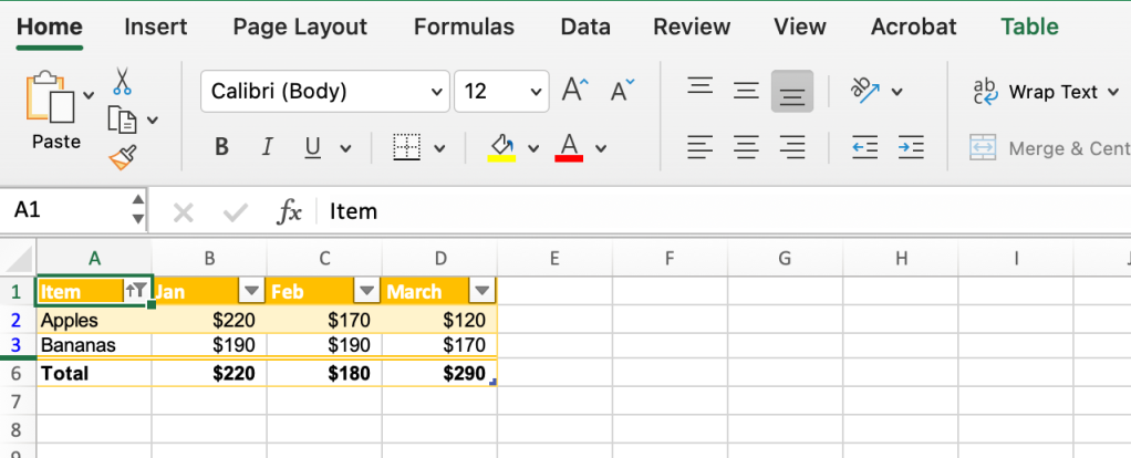
The final product looks like this:

filtered table with only Apples and Bananas rows visible

The filtered table shows only the Apples and Bananas data.

Shimon Brathwaite / IDG

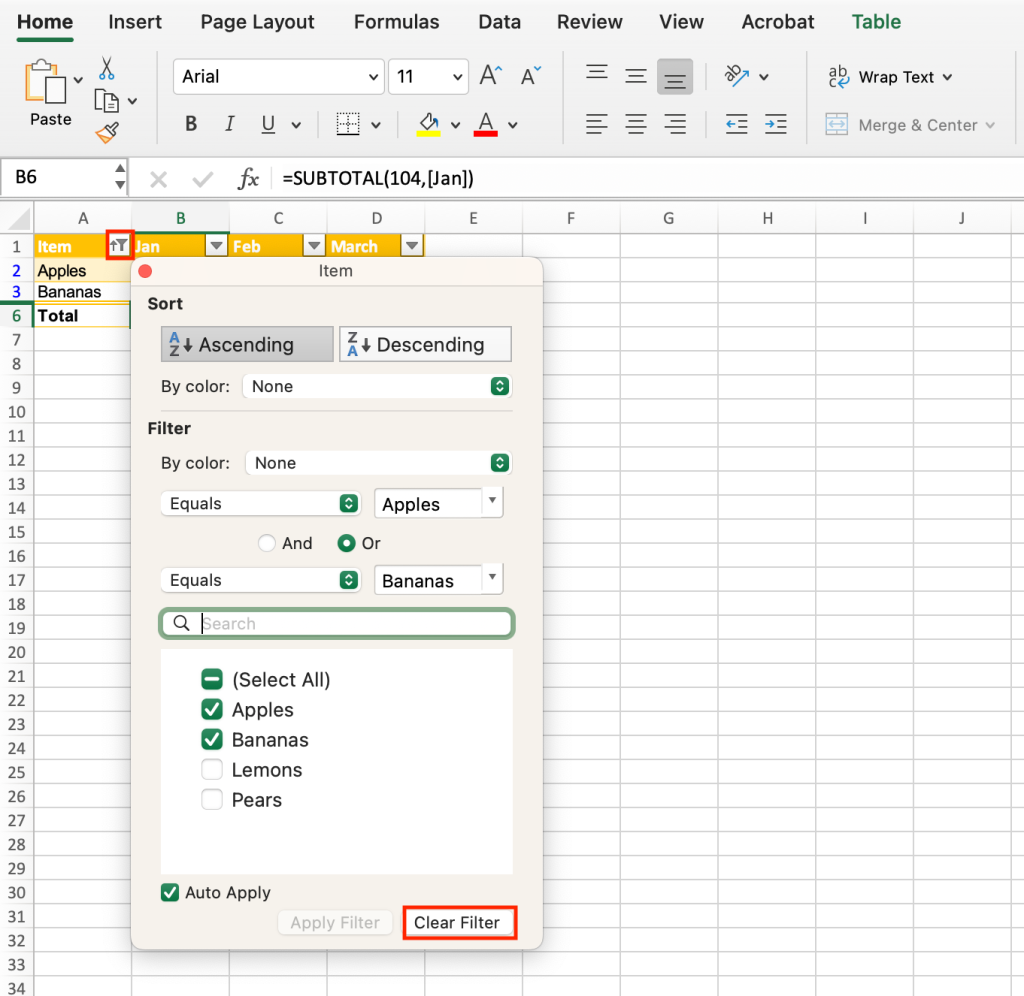
To go back to the normal view where all of the data is visible, simply click the column header button again and select Clear Filter.

clearing the filters to restore the full table data

Select Clear Filter to make all table data visible again.

Shimon Brathwaite / IDG

Tip: When you’ve sorted by a column, the button next to that column header changes to show an arrow pointing up next to the downward triangle. When you’ve filtered the items in a column, the button shows a funnel next to the triangle. And when you’ve both sorted and filtered the data, the button shows both an up arrow and a funnel. This indicator lets you know at a glance when sorting or filtering has been done to a table and which column it’s been done on.

Another way to filter is based on certain criteria, such as showing only items with numbers greater than a certain value. This is called conditional filtering. To see this in action, select the down arrow triangle to the Jan header. In the center of the pane that appears, click the first Equals dropdown and change it to Greater Than or Equal To, then type in 200 in the field to the right. Click the radio button for And. Then change the second dropdown to Less Than or Equal To and type in 300 on the right.

srcset="https://b2b-contenthub.com/wp-content/uploads/2024/06/excel-tables-09-conditional-filter.png?quality=50&strip=all 586w, https://b2b-contenthub.com/wp-content/uploads/2024/06/excel-tables-09-conditional-filter.png?resize=192%2C300&quality=50&strip=all 192w, https://b2b-contenthub.com/wp-content/uploads/2024/06/excel-tables-09-conditional-filter.png?resize=446%2C697&quality=50&strip=all 446w, https://b2b-contenthub.com/wp-content/uploads/2024/06/excel-tables-09-conditional-filter.png?resize=107%2C168&quality=50&strip=all 107w, https://b2b-contenthub.com/wp-content/uploads/2024/06/excel-tables-09-conditional-filter.png?resize=54%2C84&quality=50&strip=all 54w, https://b2b-contenthub.com/wp-content/uploads/2024/06/excel-tables-09-conditional-filter.png?resize=307%2C480&quality=50&strip=all 307w, https://b2b-contenthub.com/wp-content/uploads/2024/06/excel-tables-09-conditional-filter.png?resize=230%2C360&quality=50&strip=all 230w, https://b2b-contenthub.com/wp-content/uploads/2024/06/excel-tables-09-conditional-filter.png?resize=160%2C250&quality=50&strip=all 160w" width="586" height="916" sizes="(max-width: 586px) 100vw, 586px">

Setting two conditions for filtering a table.

Shimon Brathwaite


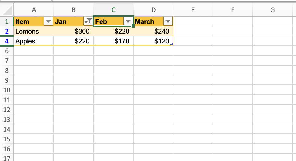
This sets the filter to show only items that have values from 200 to 300 in the Jan column, as shown below.

table with conditional filtering applied

Only the items with values between 200 and 300 in the Jan column now appear.

Shimon Brathwaite

How to create a calculated column in an Excel table

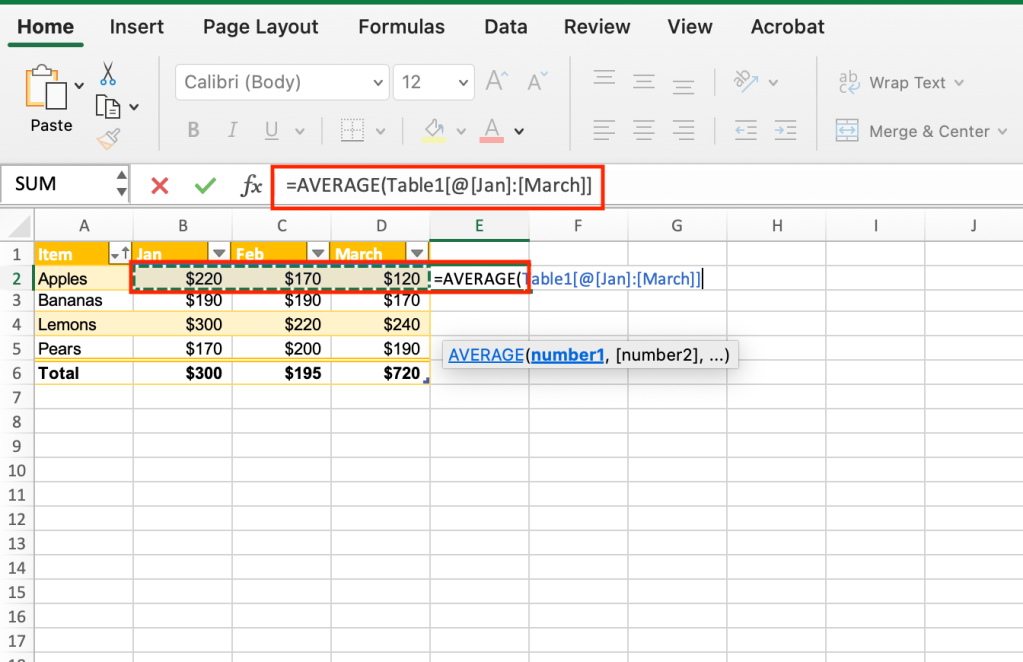
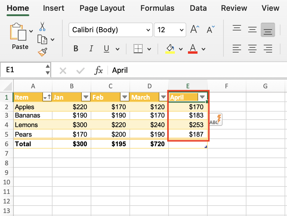
The Total row we discussed earlier calculates table data in a column, but you can also calculate data across rows. To do this easily, simply click the cell to the right of the final column in the first row of your table that contains data. Then, type in =average and select AVERAGE from the dropdown that appears. Highlight the entire row, and Excel fills in the rest of the formula to calculate the average for the values in the row. Hit Enter.

entering formula at end of row

Select AVERAGE and highlight the whole row, then press Enter.

Shimon Brathwaite


Once you hit Enter, not only will Excel calculate the average for that row, but for all of the rows in the table — and it will use formatting that is consistent with the rest of the table. Thus, you’ve created a whole column simply by entering one function. Microsoft calls these calculated columns.

calculated average column in table

Excel has calculated averages for all four rows in the table.

Shimon Brathwaite

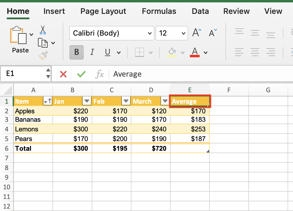
Note: Excel will typically give the new column a name in line with the other headers (in this case “April”), so you might want to rename it to something more fitting, like “Average.”

table with calculated column header changed to average

Change the column header to reflect the data being shown in the calculated column.

Shimon Brathwaite

Average isn’t the only calculation available in table rows. You can also perform sum, minimum, maximum, item count, and a host of other operations. See “How to use Excel formulas and functions” for an introduction to the functions available in Excel.

How to create a chart from a table

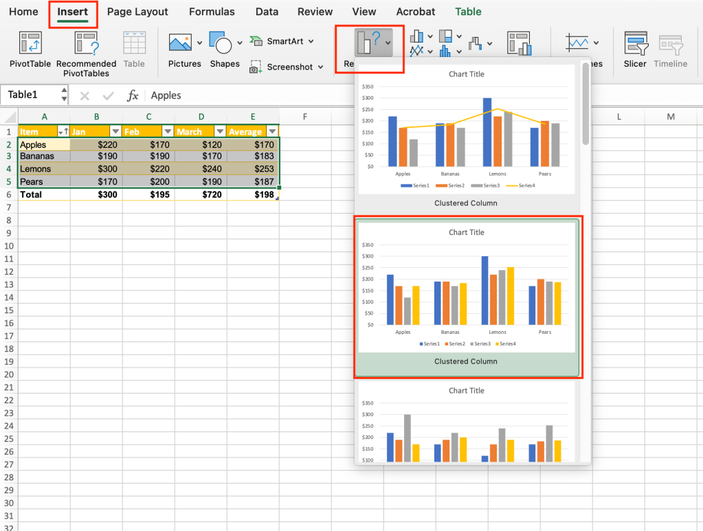
In this final section, you will learn how to make charts based on data stored in tables — a great way to visually present that data. To begin, highlight all the data rows in your table (not the header row or the Total row). Navigate to the Insert tab, select Recommended Charts, and choose the second chart — the Clustered Column chart with no line running through it.

creating a chart

Creating a chart from table data.

Shimon Brathwaite

A clustered column chart will appear on your worksheet, but you’ll notice that the labels at the bottom don’t reflect your header names. Let’s change that. Right-click the chart and choose Select Data from the menu that pops up.

On the Select Data Source screen that appears, select each legend name on the left and change it to the appropriate month by typing the month name in the Name field to the right. Once you have changed all four, click OK to apply the changes to the chart.

srcset="https://b2b-contenthub.com/wp-content/uploads/2024/06/excel-tables-15-change-labels.png?quality=50&strip=all 1036w, https://b2b-contenthub.com/wp-content/uploads/2024/06/excel-tables-15-change-labels.png?resize=278%2C300&quality=50&strip=all 278w, https://b2b-contenthub.com/wp-content/uploads/2024/06/excel-tables-15-change-labels.png?resize=768%2C829&quality=50&strip=all 768w, https://b2b-contenthub.com/wp-content/uploads/2024/06/excel-tables-15-change-labels.png?resize=949%2C1024&quality=50&strip=all 949w, https://b2b-contenthub.com/wp-content/uploads/2024/06/excel-tables-15-change-labels.png?resize=646%2C697&quality=50&strip=all 646w, https://b2b-contenthub.com/wp-content/uploads/2024/06/excel-tables-15-change-labels.png?resize=156%2C168&quality=50&strip=all 156w, https://b2b-contenthub.com/wp-content/uploads/2024/06/excel-tables-15-change-labels.png?resize=78%2C84&quality=50&strip=all 78w, https://b2b-contenthub.com/wp-content/uploads/2024/06/excel-tables-15-change-labels.png?resize=445%2C480&quality=50&strip=all 445w, https://b2b-contenthub.com/wp-content/uploads/2024/06/excel-tables-15-change-labels.png?resize=334%2C360&quality=50&strip=all 334w, https://b2b-contenthub.com/wp-content/uploads/2024/06/excel-tables-15-change-labels.png?resize=232%2C250&quality=50&strip=all 232w" width="949" height="1024" sizes="(max-width: 949px) 100vw, 949px">

You can change the legend labels manually.

Shimon Brathwaite

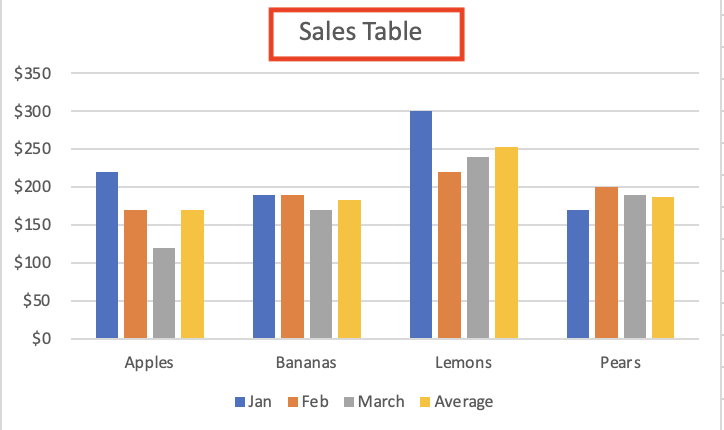
The chart now shows the correct legend labels. As a final improvement, double-click the title of the chart and rename it to “Sales Table.”

final version of chart with new title

The final chart based on our table data.

Shimon Brathwaite

Of course, you’re not limited to column charts; there are dozens of chart styles to choose from in Excel. On the Ribbon’s Insert tab to the right of Recommended Charts, you’ll find dropdowns for various styles of column charts, line charts, and pie charts, as well as an array of specialized charts such as treemap, histogram, scatter charts and more. It’s worth experimenting with different styles to see which works best to present the data or trend you want to highlight.

More Excel tutorials: